
Binary classification is a type of classification model with two class labels. For example, a spam detection model has two classes: spam and not spam. Binary classification tasks usually involve one label for a normal state and another for an abnormal state. In this article, I will take you through binary classification in machine learning with Python.
The MNIST
I will use the MNIST dataset, a set of 70,000 small images of digits handwritten by high school students and employees of the US Census Bureau. Each image is labeled with the digit it represents. This set has been studied so much that it is often called the “hello world” of machine learning.
Whenever people come up with a new classification algorithm, they are curious to see how it performs on MNIST, and anyone learning machine learning deals with this dataset sooner or later. So let's import some libraries to start our binary classification model:
# Python ≥3.5 is required
import sys
assert sys.version_info >= (3, 5)

# Scikit-Learn ≥0.20 is required
import sklearn
assert sklearn.__version__ >= "0.20"

# Common imports
import numpy as np
import os

# to make this notebook's output stable across runs
np.random.seed(42)

# To plot pretty figures
%matplotlib inline
import matplotlib as mpl
import matplotlib.pyplot as plt
mpl.rc('axes', labelsize=14)
mpl.rc('xtick', labelsize=12)
mpl.rc('ytick', labelsize=12)
Scikit-Learn provides many helper functions to download popular datasets, and MNIST is one of them. The following code fetches the MNIST dataset:
from sklearn.datasets import fetch_openml
mnist = fetch_openml('mnist_784', version=1)
mnist.keys()

Now let's look at the data:
X, y = mnist["data"], mnist["target"]
X.shape
(70000, 784)
y.shape
(70000, 784)
y.shape
(70000,)
28 * 28
784
There are 70,000 images, and each image has 784 features. This is because each image is 28 × 28 pixels, and each feature simply represents one pixel's intensity, from 0 (white) to 255 (black). Let's take a peek at one digit from the dataset. All you need to do is grab an instance's feature vector, reshape it to a 28 × 28 array, and display it with Matplotlib's imshow() function:
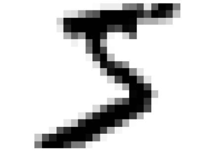
Note that the label is a string. Most machine learning algorithms expect numbers, so let's cast y to integers:
y = y.astype(np.uint8)
Now, before training the binary classification model, let's look at the digits:
def plot_digit(data):
    image = data.reshape(28, 28)
    plt.imshow(image, cmap = mpl.cm.binary,
               interpolation="nearest")
    plt.axis("off")
def plot_digits(instances, images_per_row=10, **options):
    size = 28
    images_per_row = min(len(instances), images_per_row)
    images = [instance.reshape(size,size) for instance in instances]
    n_rows = (len(instances) - 1) // images_per_row + 1
    row_images = []
    n_empty = n_rows * images_per_row - len(instances)
    images.append(np.zeros((size, size * n_empty)))
    for row in range(n_rows):
        rimages = images[row * images_per_row : (row + 1) * images_per_row]
        row_images.append(np.concatenate(rimages, axis=1))
    image = np.concatenate(row_images, axis=0)
    plt.imshow(image, cmap = mpl.cm.binary, **options)
    plt.axis("off")
plt.figure(figsize=(9,9))
example_images = X[:100]
plot_digits(example_images, images_per_row=10)
save_fig("more_digits_plot")
plt.show()
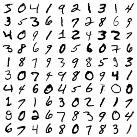
You should always create a test set and set it aside before inspecting the data closely. The MNIST dataset is already split into a training set and a test set:
X_train, X_test, y_train, y_test = X[:60000], X[60000:], y[:60000], y[60000:]
Training a binary classification model
Let's simplify the problem for now and try to identify only one digit, for example the digit 5. This “5-detector” will be an example of a binary classifier, capable of distinguishing between just two classes: 5 and not-5. Let's create the target vectors for this classification task:
y_train_5 = (y_train == 5)
y_test_5 = (y_test == 5)
Now let's pick a classification model and train it. A good place to start is Stochastic Gradient Descent (SGD), which deals with training instances independently, one at a time, as we will see later in our binary classification model. Let's build a binary classifier with SGDClassifier and train it on the whole training set:
from sklearn.linear_model import SGDClassifier

sgd_clf = SGDClassifier(max_iter=1000, tol=1e-3, random_state=42)
sgd_clf.fit(X_train, y_train_5)

sgd_clf.predict([some_digit])
array([ True])
The classifier guesses that this image represents a 5 (True). It looks like it guessed right in this particular case. Now let's evaluate the performance of our binary classification model.
Performance measures
Evaluating a classifier is often trickier than evaluating a regressor, so we will spend a larger part of this article evaluating our binary classification model.
Implementing cross-validation on the binary classification model
Sometimes you will need more control over the cross-validation process than what Scikit-Learn provides off the shelf. In these cases, you can implement cross-validation yourself. The following code does roughly the same thing as Scikit-Learn's cross_val_score() function and prints the same result:
from sklearn.model_selection import StratifiedKFold
from sklearn.base import clone

skfolds = StratifiedKFold(n_splits=3, random_state=42)

for train_index, test_index in skfolds.split(X_train, y_train_5):
    clone_clf = clone(sgd_clf)
    X_train_folds = X_train[train_index]
    y_train_folds = y_train_5[train_index]
    X_test_fold = X_train[test_index]
    y_test_fold = y_train_5[test_index]

    clone_clf.fit(X_train_folds, y_train_folds)
    y_pred = clone_clf.predict(X_test_fold)
    n_correct = sum(y_pred == y_test_fold)
    print(n_correct / len(y_pred))
0.95035
0.96035
0.9604
The StratifiedKFold class performs stratified sampling to produce folds that contain a representative ratio of each class. At each iteration, the code creates a clone of the classifier, trains that clone on the training folds and makes predictions on the test fold. It then counts the number of correct predictions and outputs the ratio of correct predictions.
Let's use the cross_val_score() function to evaluate our SGDClassifier model, using K-fold cross-validation with three folds. Remember that K-fold cross-validation means splitting the training set into K folds, then making predictions and evaluating them on each fold using a model trained on the remaining folds:
from sklearn.model_selection import cross_val_score
cross_val_score(sgd_clf, X_train, y_train_5, cv=3, scoring="accuracy")
array([0.95035, 0.96035, 0.9604 ])
Wow! Above 93% accuracy on all cross-validation folds. Well, before you get too excited, let's look at a very dumb classifier that just classifies every single image in the “not-5” class:
from sklearn.base import BaseEstimator
class Never5Classifier(BaseEstimator):
    def fit(self, X, y=None):
        pass
    def predict(self, X):
        return np.zeros((len(X), 1), dtype=bool)

never_5_clf = Never5Classifier()
cross_val_score(never_5_clf, X_train, y_train_5, cv=3, scoring="accuracy")
array([0.91125, 0.90855, 0.90915])
That's right, it has over 90% accuracy. This is simply because only about 10% of the images are 5s, so if you always guess that an image is not a 5, you will be right about 90% of the time. I hope you liked this article on the binary classification model in machine learning.


